From PCA to the Subspace Method
In the example code of this tutorial, we assume for simplicity that the following symbols are already imported.
import matplotlib.pyplot as plt
import numpy as np
from matplotlib.colors import ListedColormap

from sklearn.datasets import make_moons, make_circles, make_classification
from sklearn.model_selection import train_test_split
from sklearn.discriminant_analysis import LinearDiscriminantAnalysis
from sklearn.metrics import accuracy_score

import sys, os, numpy as np
import matplotlib.pyplot as plt, seaborn as sns
sys.path.insert(0, os.pardir)
import warnings
warnings.filterwarnings('ignore')

from cvt.models import SubspaceMethod
In this example we will start with principal component analysis (PCA) and work our way to classification with the subspace method (SM).
We will conduct the procedure in the following steps.
Prepare a dataset
Peform PCA on each class and select eigenvectors (Training)
Calculate cosine similarities for each subspace (Classification)
Bad use case for SM
Good use case for SM
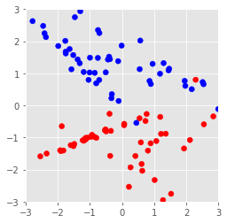
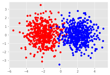
1. Prepare a dataset
Here we create a random set of data with 2 features.
The make_classification function generates data for a random n-class
classification problem.
plt.style.use('ggplot')

# Create a random set of data of 2 dimensions
X, y = make_classification(n_features=2, n_redundant=0)

# Plot the dataset
cm_bright = ListedColormap(['#FF0000', '#0000FF'])
plt.scatter(*X.T, c=y,cmap=cm_bright)
plt.xlim(-3,3)
plt.ylim(-3,3)
plt.axes().set_aspect('equal')
plt.show()
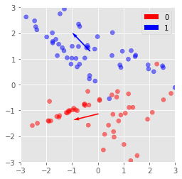
2. Peform PCA on each class and select eigenvectors (Training)
In most cases of the subspace method, PCA is performed on each class to create subspaces. These subspaces are then used as references to determine the class of newly introduced data.
In this example, we have only 2 dimensions. Therefore we will choose a 1 dimensional subspace to use for classification.
This 1-dimensional subspace will determined with pca, so it will be the direction which captures the largest variance.
def pca(X, n_components):
    """
    Tip from https://stackoverflow.com/a/45435548

    np.eigh guarantees you that the eigenvalues are sorted and
    uses a faster algorithm that takes advantage of the fact
    that the matrix is symmetric.
    If you know that your matrix is symmetric, use this function.
    """

    eig_vals, eig_vecs = np.linalg.eigh(X.T@X)
    return eig_vals[::-1][:n_components], eig_vecs[::-1][:n_components]

dct = {}
for c in range(2):
    Xc = X[np.where(y==c)]
    _, eig_vecs = pca(Xc, 1)

    # Store subspaces to use later for classification
    dct[c] = eig_vecs

    print(f'Eigen vectors from class {c:.0f}:\n{eig_vecs}\n')
    plt.quiver(*Xc.mean(axis=0), eig_vecs[0][0],eig_vecs[0][1], label=c,
               color=cm_bright(c), scale=1, angles='xy', scale_units='xy')

plt.scatter(*X.T, c=y, cmap=cm_bright, alpha=0.5)
plt.xlim(-3,3)
plt.ylim(-3,3)
plt.axes().set_aspect('equal')
plt.legend()
plt.show()
Eigen vectors from class 0:
[[-0.97085135 -0.23968241]]

Eigen vectors from class 1:
[[-0.69337618  0.7205758 ]]
3. Calculate cosine similarities for each subspace (Classification)
Next, to classify data we calculate the cosine similarities between the input vector and each subspace.

image.png
The cosine similarity can be interpreted as
The projection legngth from the input vector to the subspace
The “angle” between the input vector and a subspace
or if we change our perspective the cosine similarity is inversely related to
The rejection legngth from the input vector to the subspace
Below is an example using the subspaces calculated from the previous data.
test_x = [1, -1]

fig, axs = plt.subplots(ncols=2)

for c, subspace in dct.items():
    m = subspace[0][0] / subspace[0][1]
    xs = np.linspace(-3,3)
    ys = m * xs

    # cos_sim = cos(θ)
    # = (eigen_vec, test_x)/|eigen_vec||test_x|
    cos_sim = np.linalg.norm(dct[c] @ test_x)
    theta = np.arccos(cos_sim)
    dist = np.sin(theta) * np.linalg.norm(test_x)
    print(f'Class {c}: cosine similarity={cos_sim:.3f}, angle={np.rad2deg(theta):.3f}, rejection length={dist:.3f}')


    axs[c].quiver(0,0,*test_x, color='green', label='test_x', scale_units='xy',angles='xy',scale=1)
    axs[c].plot(xs, ys, color=cm_bright(c), label=c)
    axs[c].set_xlim(-3,3)
    axs[c].set_ylim(-3,3)
    axs[c].set_aspect('equal')
    axs[c].legend()

y_pred = 0 if np.linalg.norm(dct[0] @ test_x) > np.linalg.norm(dct[1] @ test_x) else 1
print(f'test_x will be classified to {y_pred}')
plt.show()
Class 0: cosine similarity=0.731, angle=43.016, rejection length=0.965
Class 1: cosine similarity=1.414, angle=nan, rejection length=nan
test_x will be classified to 1

Now that we understand the subspace method, lets classify the data we used to generate the subspaces to see how well our classifier works.
score = 0

for i in range(len(X)):
    x = X[i]
    y_gt = y[i] # ground truth label

    # calculate projection distance to the
    # first classes subspace
    proj1 = np.linalg.norm(dct[0] @ x)

    # calculate projection distance to the
    # second classes subspace
    proj2 = np.linalg.norm(dct[1] @ x)

    assert proj1 != proj2, 'Tie!'
    y_pred = 0 if proj1 > proj2 else 1

    score += 1 if y_pred == y_gt else 0

print(score / len(y))
0.62
The results do not look good.
Why could this be?
Let’s have a look at the decision boundary to understand what is going on.
# This can be resused to visualize boundaries of other classifiers
def plot_decision_boundaries(clf, X, y, h=0.01, show=True):
    fig, ax = plt.subplots()

    # Build mesh
    x_min, x_max = X[:, 0].min() - .5, X[:, 0].max() + .5
    y_min, y_max = X[:, 1].min() - .5, X[:, 1].max() + .5
    xx, yy = np.meshgrid(np.arange(x_min, x_max, h),
                         np.arange(y_min, y_max, h))

    # Plot the decision boundary. For that, we will assign a color to each
    # point in the mesh [x_min, x_max]x[y_min, y_max].
    Z = clf.predict_proba(np.c_[xx.ravel(), yy.ravel()])[:, 1]

    # Put the result into a color plot
    cm = plt.cm.RdBu
    Z = Z.reshape(xx.shape)
    ax.contourf(xx, yy, Z, cmap=cm, alpha=.8)

    cm_bright = ListedColormap(['#FF0000', '#0000FF'])
    ax.scatter(*X.T, c=y, cmap=cm_bright, edgecolors='k')
    ax.set_title(f'Score={clf.score(X,y)}')

    if show:
        plt.show()
    else:
        return fig, ax

# Using the API provided in this package, we can easily create a subspace classifier.
def format_input(X, y):
    X = [X[np.where(y==t)] for t in np.unique(y)]
    return X, np.unique(y)

smc = SubspaceMethod(n_subdims=1, faster_mode=True)
smc.fit(*format_input(X, y))
smc.score(X, y)

fig, ax = plot_decision_boundaries(smc, X, y, show=False)

ax.set_aspect('equal')
ax.quiver(0,0,*smc.dic[0],angles='xy', scale_units='xy',scale=1, color='#FF0000')
ax.quiver(0,0,*smc.dic[1],angles='xy', scale_units='xy',scale=1, color='#0000FF')
plt.show()
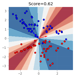
As you can see, the subspace method is not very good with discriminating classes in a low dimensional space.
This is because the subspace method is “dimensionally hungry”, it works much better in high dimensional data.
Many classification problems assume that the data given can be represented in a much lower dimension, the subspace method is a typical example.
Another point to make is that the subspace method works especially well on class that have a fundamentally different structure. On the otherhand it does not work when the structure of the distributions are similar.
In the next sections, I will give a bad use case for SM and a good use case.
4. Bad use case for SM
Here I will give a bad use case for SM. In essence they both have the same anti-pattern, that is, the generated subspaces are equal. Classification with subspaces becomes very difficult when the subspaces generated from pca are too similar.
An easy example on the 2 dimensional plane is when classes have data a distribution with the same covariance matrix.
Consider the following data:
X_ = np.append(
    np.random.normal(loc=(-2, 0), size=(500, 2)),
    np.random.normal(loc=(2, 0), size=(500, 2)), axis=0)

y_ = np.append(
    np.zeros(500),
    np.ones(500))

plt.scatter(*X_.T, c=y_, cmap=cm_bright)
plt.axes().set_aspect('equal')
plt.show()
If we conduct pca onto these distribution we should get a very similar eigenvectors.
for c in np.unique(y_):
    eig_vals, eig_vecs = pca(X_[np.where(y_==c)], 1)
    print(f'Eigen vectors from class {c:.0f}:\n{eig_vecs}\n')
Eigen vectors from class 0:
[[-0.99959599  0.02842293]]

Eigen vectors from class 1:
[[-0.99955934  0.02968376]]
Obviously the resulting classifier is not very good.
smc = SubspaceMethod(n_subdims=1, faster_mode=True)
smc.fit(*format_input(X_, y_))
smc.score(X_, y_)
0.524
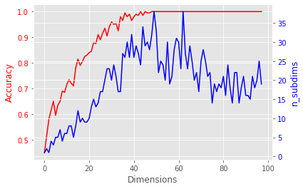
5. Good use case for SM
The subspace method becomes more powerful in higher dimensions.
I will demonstrate this by generating toy data in high dimensions and apply the subspace method to it.
scores = []
n_subdims = []
for d in range(2, 100):
    X_, y_ = make_classification(n_samples=200, n_features=d, n_redundant=0)

    # Exhaustive search for the optimal subspace dimension
    max_score = (0, 0) # store n_subdims and score
    for n in range(1, d):
        smc = SubspaceMethod(n_subdims=n, faster_mode=True)
        smc.fit(*format_input(X_, y_))
        score = smc.score(X_, y_)
        max_score = (n, score) if max_score[1] < score else max_score

    n_subdims.append(max_score[0])
    scores.append(max_score[1])
fig, ax1 = plt.subplots()
ax2 = ax1.twinx()

ax1.plot(scores, color='red')
ax1.set_xlabel('Dimensions')
ax1.set_ylabel('Accuracy', color='red')
ax1.tick_params(axis='y', labelcolor='red')

ax2.plot(n_subdims, color='blue', label='n_subdims')
ax2.set_ylabel('n_subdims', color='blue')
ax2.tick_params(axis='y', labelcolor='blue')

plt.show()