Constrained Subspace Method
Summary
The Constrained Mutual Subspace Method (CMSM) is an extension of the Mutual Subspace Method (MSM) [FY05]. In CMSM, we project the input subspace and the reference subspace onto the General Difference Subspace (GDS). This step is useful to extract effective features for classification [NYF05].
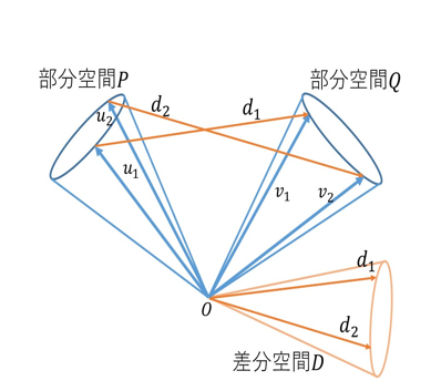
Fig.1
General Difference Subspace (GDS)
A difference space can be defined between two subspaces, just as a difference vector exists between two vectors (See fig 2.). The difference space is a subspace containing the difference vector \(d_i\) between the \(i_{th}\) canonical vectors of subspaces \(\mathcal{P}\) and \(\mathcal{Q}\), i.e. \(u_i\) and \(v_i\).
The General Difference Subspace (GDS) is not the differece subspace between two only subspaces, but instead a differece subspace of multiple subspaces [FM15].
A projection to the GDS usually results in an increase of orthoganality between subspaces. Furthermore, the projection of vector data onto the GDS can increase the Fisher discrimination ratio, and can perform feature extraction effective for discrimination.

Calculation of GDS
Let \(\Phi^C=[\phi_1^C,\phi_d^C]\) be the \(d\)-dimensional orthogonal bais vectors of the subspace of class \(C\). The GDS can be obtained by applying eigendecomposition to the following matrix \(G\).
When projecting data onto the generalized difference subspace, if the number of dimensions g is (the number of classes -1), the Fisher discrimination ratio of the projected data is maximized.
The number of dimensions g of the generalized difference subspace is determined by the number of eigenvectors extracted from W.
Constrained MSM (CMSM)
In Constrained MSM (CMSM), a constrained subspace \(\mathcal{C}\) is introduced. \(\mathcal{C}\) is a ideally a subspace which includes the effective components for recognition and does not include any unnecessary components such as undersirable variation. Usually, the GDS is used as \(\mathcal{C}\).
Learning Phase
Generate \(k\) class subspaces from each class by using PCA.
Generate a GDS using the generate class subspaces.
Project the training data onto the GDS.
Generate \(k\) class subspaces using the projected data and PCA.
Recognition Phase
Project the input data onto the GDS abd generate the input subspace \(\mathcal{P}\).
Calculate \(S\) (or \(\tilde{S}\)) between \(\mathcal{P}\) and each subspace \(\mathcal{Q}\).
Classify \(\mathcal{P}\) into the class where \(S\) (or \(\tilde{S}\)) was calculated to be the highest.
Also, you may add a rejection thershold on \(S\) (or \(\tilde{S}\)) to reject classifications with low similarity.